Direct Conditional Parameterization for N-Dimensional Splatting (NeurIPS 2026)

Abstract

N-dimensional splatting extends 3D Gaussian Splatting with conditioning variables such as view direction and time to model view-dependent and dynamic effects. Each primitive is lifted into a joint distribution over 3D position and conditioning variables, and at render time is conditionally sliced at the query to recover a 3D primitive whose mean, opacity, and covariance vary continuously with view or time.

N-DGS (covering 6DGS and 7DGS) and UBS together represent the leading N-dimensional splatting formulations across Gaussian and Beta kernels, but share the same conditional-slicing step: all three effects are derived from the joint covariance matrix per primitive in every forward pass, requiring matrix inversions and regression-matrix multiplications that scale with primitive count. The conditional-slicing step is kernel-agnostic, so a single improvement carries across families.

We introduce direct conditional parameterization, replacing the covariance-derived form with explicit per-effect parameters: a Cholesky precision factor for opacity and a displacement matrix with learnable per-dimension coupling for position. Applied to both kernels, the parameterization yields dGS (Gaussian) and dBS (Beta). Across five static and dynamic benchmarks, dGS and dBS match or exceed their covariance-derived counterparts on quality (up to +1.26 dB in the main MCMC evaluation) while running 6.9–7.7× faster at the slicing step and up to 2.66× faster end-to-end rendering. Direct conditioning is a kernel-agnostic drop-in replacement for covariance-derived conditioning in N-dimensional splatting.

How It Works

Rendering only needs three things from a joint primitive: the query precision, the query-to-position regression, and the conditional spatial covariance. We parameterize them directly instead of deriving them from an ambient joint covariance through inversion and Schur complements.

dGS pipeline: direct precision opacity decay, learnable coupling control, and spatially scaled coupling factor

Opacity · L

Direct precision factor

A lower-triangular Cholesky factor makes V_qq = LL^⊤ the precision itself. Opacity is one triangular product and a squared norm, with no inversion.

Coupling · Λ

Learnable per-dimension coupling

Λ ∈ [0,1]^C decides how much each query dimension moves the mean. 0 decouples position from opacity; 1 recovers full N-DGS-style coupling.

Position · V_pq

Spatially scaled coupling factor

V_pq = s̄Θ_pq ties the shift to the primitive's mean scale. Removing this prior costs 2.65–2.97 dB.

Direct conditioning, given the query deviation δ = q − μ_q:

Opacity α_cond = α · exp( −λ_o · ‖ L^⊤δ ‖² )

Position μ_cond = μ_p + V_pq · diag(Λ) · V_qq · δ

The conditional covariance stays query-independent, as in 3DGS, so existing densification strategies carry over unchanged. For the Beta kernel (dBS), the opacity decay becomes ∏_i (1 − tanh(z_i²))^β_i with z = L^⊤δ, and the same bandwidth β supplies the coupling Λ_β = min(β/4, 1). We also prove the unrestricted tuple is a smooth, globally bijective coordinate chart for joint Gaussian covariances.

What the slicing step no longer computes

Per-primitive operation	N-DGS	UBS	dGS	dBS
Invert Σ_qq	✓	✓	—	—
Regression matrix Σ_pqΣ_qq⁻¹	✓	✓	—	—
Covariance correction	✓	✓	—	—
Slicing time, C=3 (view)	0.71 ms	0.67 ms	0.10 ms (7.1×)	0.10 ms (6.9×)
Slicing time, C=4 (view + time)	0.96 ms	1.34 ms	0.12 ms (7.7×)	0.13 ms (7.2×)

Slicing-only CUDA forward pass, 1M Gaussians, NVIDIA A100. Speedups are over the covariance-derived counterpart.

Quantitative Results

MCMC densification with matched Gaussian budgets. Each direct method is paired with its covariance-derived counterpart, so any difference reflects the conditioning parameterization alone.

Dataset	Method	#Gauss (K)	Time (m)↓	FPS↑	FPS_CUDA↑	PSNR↑	SSIM↑	LPIPS↓
NeRF Syntheticstatic	N-DGS	300	10.43	183.58	348.95	34.04	0.973	0.027
	dGS	300	10.26	245.18	593.94	34.34	0.973	0.026
	UBS	300	6.80	155.96	306.33	34.48	0.975	0.026
	dBS	300	5.48	239.09	415.66	34.53	0.975	0.025
Mip-NeRF 360static	N-DGS	2,852	51.23	35.69	75.31	26.88	0.775	0.263
	dGS	2,574	49.85	42.49	200.56	27.67	0.794	0.227
	UBS	3,057	28.59	40.94	76.18	28.50	0.841	0.183
	dBS	3,057	24.42	62.05	157.45	28.70	0.842	0.185
6DGS-PBRstatic	N-DGS	163	54.80	328.75	476.79	40.06	0.976	0.039
	dGS	163	47.54	356.15	551.02	40.34	0.976	0.038
	UBS	163	8.70	239.87	348.63	39.53	0.975	0.042
	dBS	163	8.47	305.33	401.93	39.72	0.976	0.042
D-NeRFdynamic	N-DGS	150	10.31	306.51	501.52	34.63	0.976	0.033
	dGS	150	10.61	407.40	746.65	34.64	0.976	0.030
	UBS	150	8.37	229.83	371.81	32.91	0.967	0.040
	dBS	150	9.34	323.75	463.09	33.55	0.972	0.033
7DGS-PBRdynamic	N-DGS	175	28.44	294.48	511.12	29.20	0.944	0.063
	dGS	175	31.12	366.06	577.38	29.90	0.948	0.061
	UBS	175	9.90	232.17	396.33	30.61	0.951	0.057
	dBS	175	8.79	347.93	539.57	31.87	0.955	0.053

Means over all scenes. FPS uses a PyTorch reference slicer; FPS_CUDA uses the fused CUDA slicing kernel. Bold = better of each pair. All methods: NVIDIA A100, 30K iterations, TC-GS rasterizer, identical learning rates and densification schedules per dataset.

Comparison with state-of-the-art static-scene methods

dBS achieves the best PSNR on Mip-NeRF 360 (28.70 dB) and ties for best PSNR on NeRF Synthetic (34.53 dB). UBS and dBS are re-evaluated under the 3DGS protocol, so UBS numbers differ from the original paper.

	Method	Mip-NeRF 360			NeRF Synthetic
	Method	PSNR↑	SSIM↑	LPIPS↓	PSNR↑	SSIM↑	LPIPS↓
Implicit	Instant-NGP	25.51	0.684	0.398	33.18	0.959	0.055
	Mip-NeRF 360	27.69	0.792	0.237	33.25	0.962	0.039
	Zip-NeRF	28.54	0.828	0.189	33.10	0.971	0.031
Explicit	3DGS	27.20	0.815	0.214	33.31	0.969	0.037
	GES	26.91	0.794	0.250	–	–	–
	2DGS	27.04	0.805	0.297	33.07	–	–
	Mip-Splatting	27.79	0.827	0.203	33.33	0.969	0.039
	3DGS-MCMC	28.29	0.840	0.210	33.80	0.970	0.040
	DRKS	26.76	0.787	0.236	33.82	–	–
	Textured GS	27.35	0.827	0.186	33.24	0.967	0.043
	Quadratic GS	27.39	0.813	0.213	–	–	–
	Disc-GS	28.01	0.833	0.189	–	–	–
	Triangle Splatting	27.00	0.808	0.231	–	–	–
	Radiance Meshes	27.15	0.810	0.274	–	–	–
	Spherical Voronoi	28.57	0.835	0.230	34.53	0.973	0.032
	UBS	28.50	0.841	0.183	34.48	0.975	0.026
	dBS (Ours)	28.70	0.842	0.185	34.53	0.975	0.025

Bold = best, underline = second best.

Ablation: coupling and spatial scaling

Learned Λ beats both fixed extremes. Diffuse scenes prefer weak coupling and specular scenes prefer strong coupling, so the right amount is scene- and primitive-dependent.

Config	NeRF Synthetic			6DGS-PBR
Config	PSNR↑	SSIM↑	LPIPS↓	PSNR↑	SSIM↑	LPIPS↓
Λ = 0 (dGS-O, opacity only)	33.84	0.971	0.030	36.54	0.965	0.059
Λ = 1 (fixed full coupling)	33.78	0.971	0.029	37.31	0.972	0.053
dGS w/o spatial scaling s̄	31.26	0.957	0.046	34.78	0.951	0.075
Learned Λ (dGS)	33.91	0.972	0.029	37.75	0.972	0.052

Standard 3DGS densification. An unscaled coupling factor is worse than no position regression at all.

Qualitative Comparison

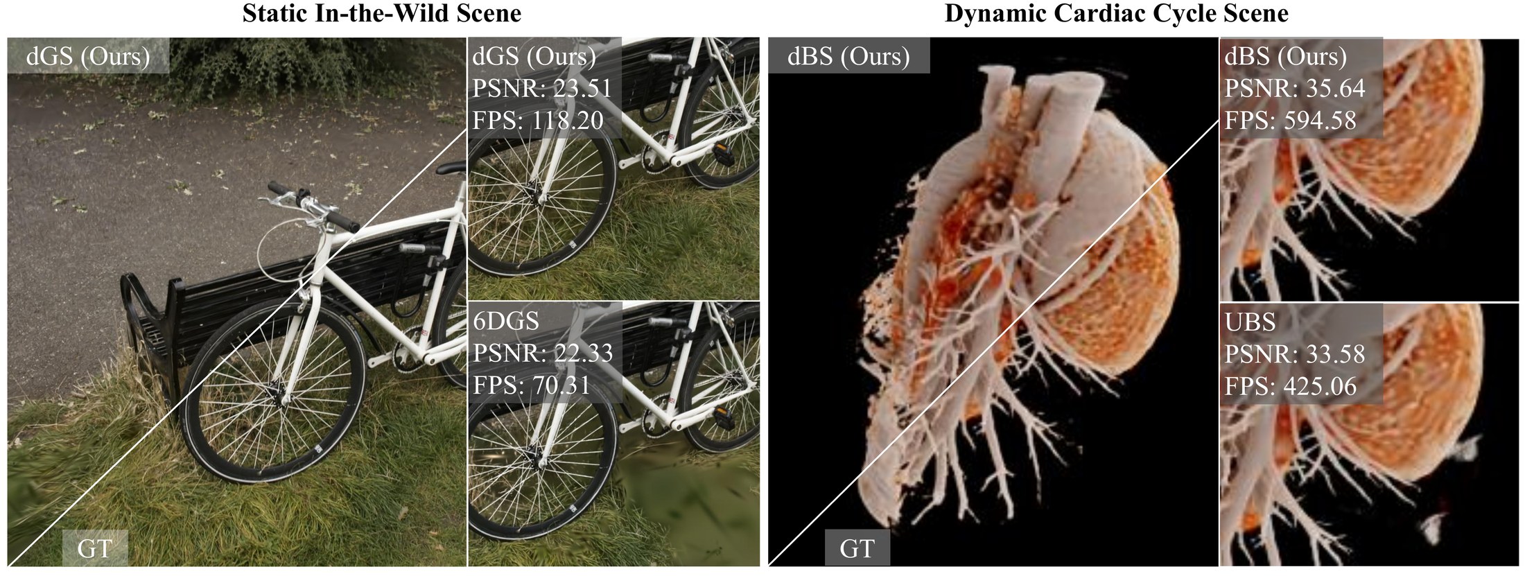
Static and dynamic scenes. dGS shows noticeably fewer artifacts than N-DGS on static scenes. On dynamic scenes, dGS and dBS both look better than their covariance-derived counterparts.

The N-Dimensional Splatting Line

BibTeX

@inproceedings{gao2026direct,
  title     = {Direct Conditional Parameterization for N-Dimensional Splatting},
  author    = {Gao, Zhongpai and Planche, Benjamin and Nguyen, Van Nguyen and Zheng, Meng and
               Choudhuri, Anwesa and Innanje, Arun and Chen, Terrence and Wu, Ziyan},
  booktitle = {Advances in Neural Information Processing Systems (NeurIPS)},
  year      = {2026}
}

Direct Conditional Parameterization for N-Dimensional Splatting

Direct conditioning improves both kernels. dGS beats 6DGS on the static bicycle scene (+1.18 dB, 1.7× FPS), and dBS beats UBS on the dynamic cardiac heart1 scene (+2.06 dB, 1.4× FPS).